Disclaimer:

This tutorial is based on the Masterclass Nick gave in Soest. Credits to him!

Level: expert

In order to get this done, you will need quite some understanding about google sheets/excel formula's.

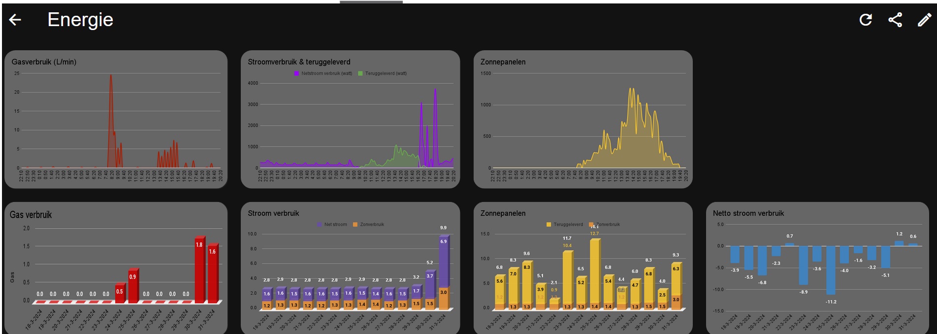
Why are we doing this?

To get very nice graphs in our dashboards!

Let's get started!

Google Sheets offers a convenient feature: forms. These forms allow you to collect data seamlessly and organize it neatly in your Google Sheets. Below is a step-by-step guide on how to create a form, link it to Google Sheets, and manage your data effectively.

Step 0: Decide how to get the numbers into google sheets

Homey has an app which can transport information into sheets. It has some API limits and doesnt trigger scripts. Also, When API limits are reached, information might be gone instead of stored into forms.

If you decide to use the homey sheets app, please skip step 1 and 2. The app will be good enough for most cases. This tutorial isnt really made for that app though.

Step 1: Making forms

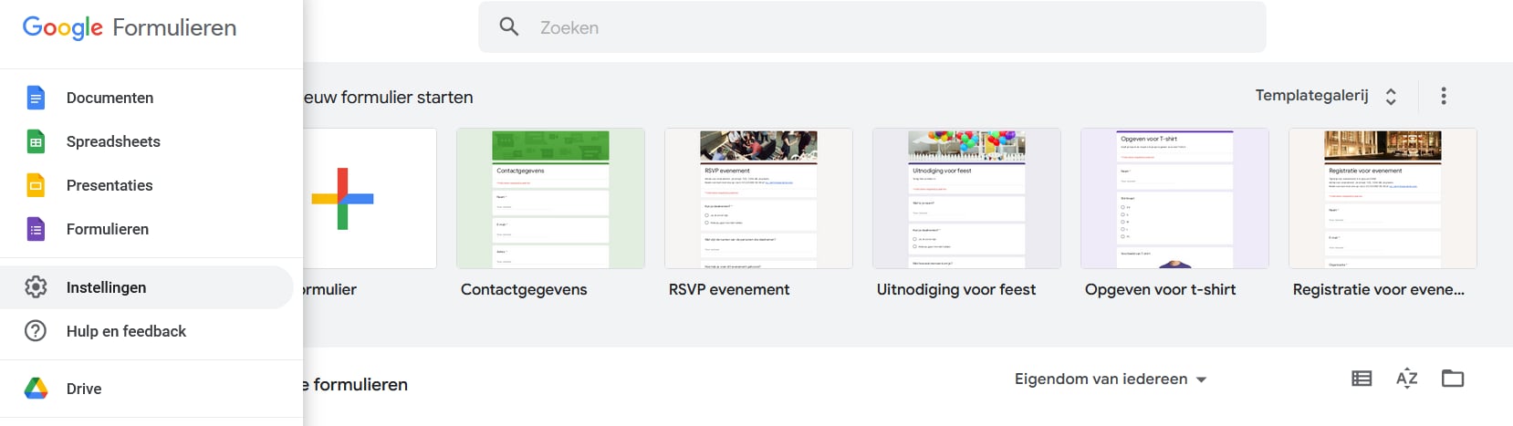
• Access Google Forms: Navigate to Google Forms by visiting https://docs.google.com/forms/ or via the Google Apps menu if you're already signed into your Google account. Create a New Form: Click on the "+ Blank" button to start a new form.

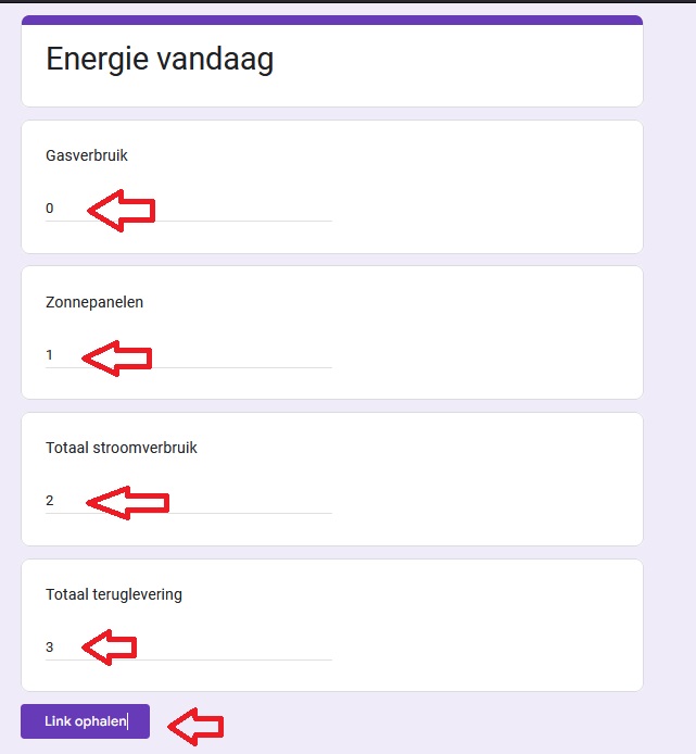
• Give your form a title by clicking on "Untitled form" at the top (In this case "Energie vandaag".
• Add Questions: Begin by adding questions. Each question you add will become a column header in your Google Sheets later on. Click on the "+ Add question" button to add questions. Choose the type of question: short answer. The form in the picture has 4 questions: "gasverbruik", "Zonnepanelen" , "Totaal stroomverbruik" and "totaal teruglevering". Continue adding questions until you have included all the information you need.

Step 2: Getting the data from Forms to Sheets

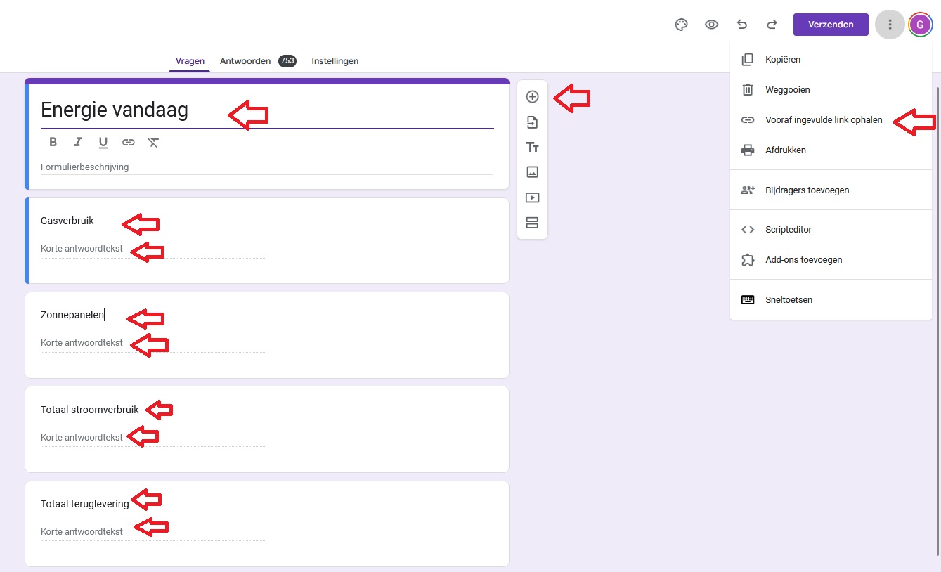
• Configure Responses: Once you've added all your questions, you can configure how responses are collected. Click on the three dots in the upper right corner and select "Get pre-filled link" (picture above). This will generate a link where you can fill in sample responses for testing purposes. Retrieve the Form Link: After filling in sample responses, click on "Get link" to generate a link to your form. Copy this link to your clipboard. In the example i filled in "0", "1", "2" and "3" as samples.

• Modify the Form Link: Open a text editor or word processor. Paste the form link. Before modifying the link, make sure you have a copy of the link as you need it later on.
• In homey, select the post request card.
• In the first part of the link, replace "/viewform" in the URL with "/formResponse" and cut the link there. You ll fill it at the place you see in the screenshot: https://docs.google.com/forms/d/e/xxxxxxxxxxxxxxxxxxxxxxx/formResponse. Where xxxxxxxxxxxxxxxxxxxxxxx is your personal code. Please keep that code origional. That part of the link can be put on 'URL'.
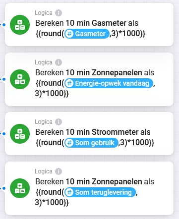
• In the second part of the link, replace the sample numbers (in my case "0, 1, 2, 3") with the number tags you want to send to google sheets. The last part will start with &entry. and will end with a tag. The tag will be the number that you want to send to google sheets*. You are able to enter all entry's behind eachother like the screenshot does. Those entry's can be filled in under 'body'. In the screenshot, i send the following tags to sheets: "10 min Gasmeter", "10 in Stroommeter", "10 min Zonnepanelen" and "10 min teruglevering".
• Under 'headers', type: Content-Type:application/x-www-form-urlencoded
• For the first part, choose: POST.

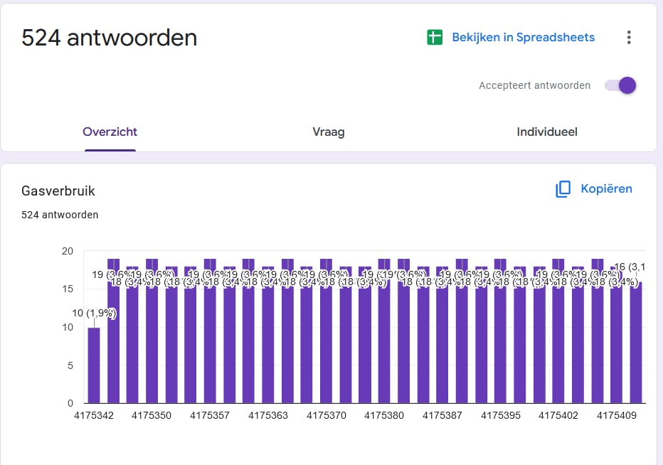
• Prepare Google Sheets: Create a new Google Sheets document where you want to store the form responses. Link Responses to Google Sheets: Go back to your Google Form. Click on the responses/answer tab at the top. Click on the green Sheets icon to link your form to a Google Sheets document. Select the Google Sheets document you prepared earlier. This will automatically populate the spreadsheet with responses as they come in.

• Note: Keep in mind that you need to send whole numbers. Homey uses "." instead of "," as a decimal separator. The graphs will need a ",". You could multiply the answers by 10, 100, or 1000 in Homey and then round them before sending them to sheets. Once in sheets, you can automatically divide the answer 10, 100, or 1000, so it has 1, 2, or 3 decimal places again. Example:

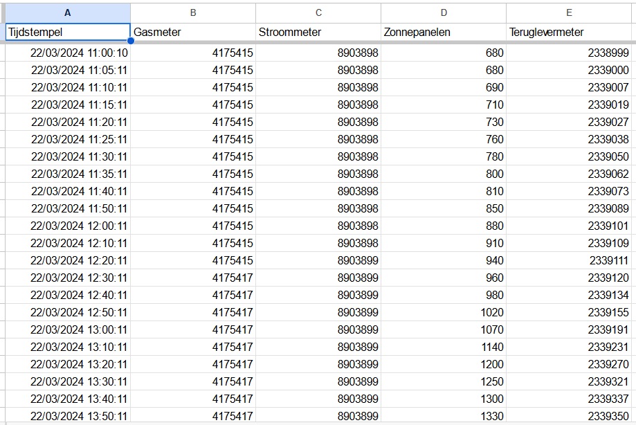
Once done, data will get into sheets like this:

Step 3: modify the data

I personally want to keep the sheet from google forms clean, so i added a new sheet by pressing the "+" at the left bottom.

To get the data of column A into the other sheet, i use the next formula:

=ARRAYFORMULA('Formulierreacties 1'!A2:A)

I multiplied all numbers by 1000 before rounding it and sending it over, i want to devide column B, C etc. Those formula's look like this:

=ARRAYFORMULA('Formulierreacties 1'!B2:B/1000)

Note: Replace 'Formulierreacties 1' if you name your sheet differently.

Here are a couple of formula's that you might want to use. Examples all have the timestamp/date in colum A and the data in colum B:

* Show all the data of month 1 (januari) of this year: =FILTER(A:B, MONTH(A:A) =1, YEAR(A:A) = YEAR(TODAY()))

* Show all the data of week 1 of this year: =FILTER(A:H, WEEKNUM(A:A) = 1, YEAR(A:A) = YEAR(TODAY()))

* Show all data of the year 2024: =FILTER(A:B, YEAR(A:A) = 2024)

* show all data of the current month: =FILTER(B:H, MONTH(A:A) = MONTH(TODAY()))

* Show all data of the current week in this year (where the week starts on monday): =FILTER(A:H, WEEKNUM(A:A, 2) = WEEKNUM(TODAY(), 2) * (YEAR(A:A) = YEAR(TODAY())))

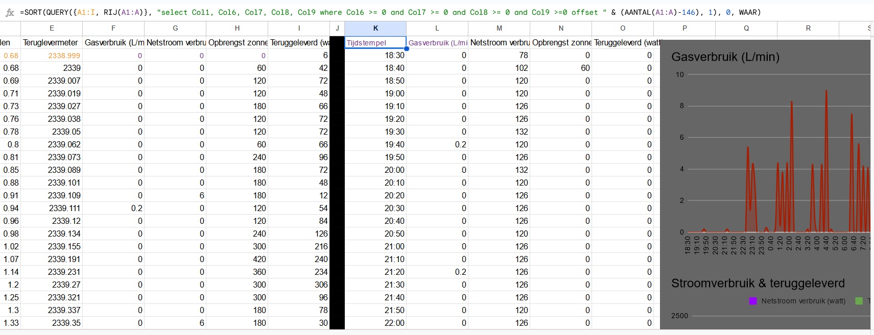
In order to show only the last 146 items: that can be done by the next Formula:

=SORT(QUERY({A1:I\ row (A1:A)}; "select Col1, Col6, Col7, Col8, Col9 offset " & (COUNT(A1:A)-146); 1); 0; TRUE)

Note: A1:l is the range of the data which has to be adjusted for your amount of columns.

Note: Rij A1:A is the row where it makes the selection.

Note: "select col 1, col6" etc. are the columns that will be displayed right of the formula where Col1 is A and Col 6 is F.

Note: "-146" is the amount of rows it displays. In this case the last rows.

Note: the, 1 makes it show the header, you could change it to 0 if you dont want it.

You could add "where Col6 >=0" if all negatieve numbers should be 0:

=SORT(QUERY({A1:I\ row (A1:A)}; "select Col1, Col6, Col7, Col8, Col9 where Col6 >= 0 and Col7 >= 0 and Col8 >= 0 and Col9 >=0 offset " & (COUNT(A1:A)-146); 1); 0; TRUE)

• Please note: ChatGPT is your friend if you need to adjust your formula.
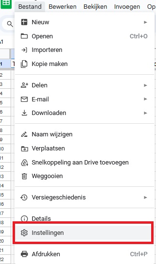
• Please note: set your language to english if you want to copy my formula (under options):

Step 4 (optional): cleaning sheets

In quite some cases, you might want to clean the sheet, for example when you d like to see a graph, starting at 00:00 and ending at 23.59. That can be done by doing the following:

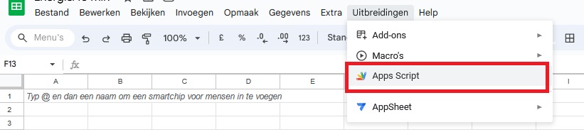
• Create an Apps Script via Menu "Extension/Apps Script" in Google Sheets.

• Copy 1 of the 2 codes:

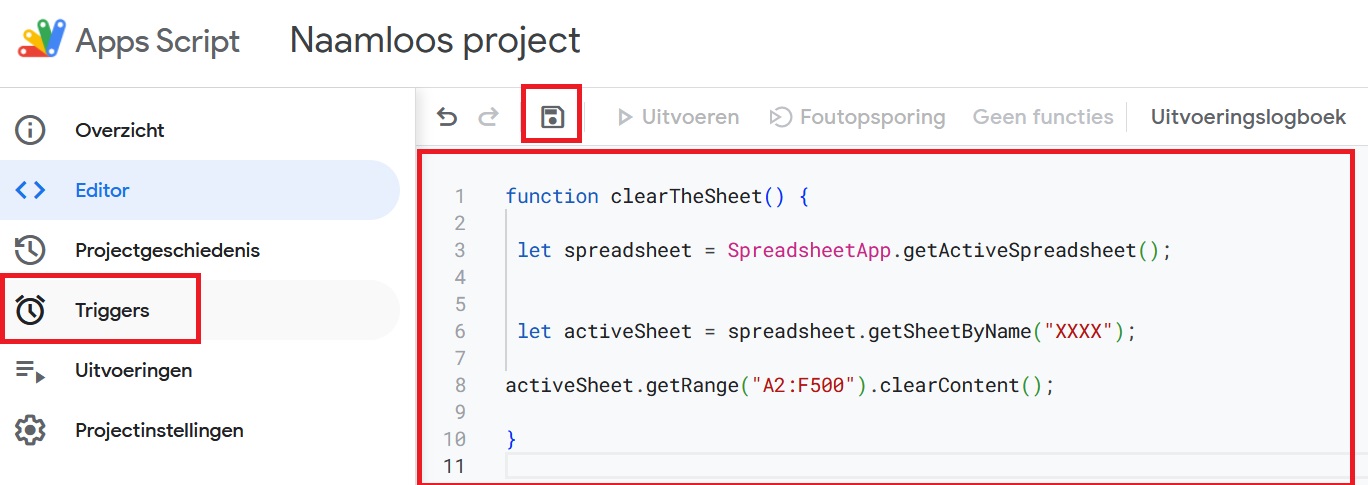
1. This clears the content of the sheet called "XXXX" from row 2 to 500. I leave the first row as column title:

function clearTheSheet() {

let spreadsheet = SpreadsheetApp.getActiveSpreadsheet();

let activeSheet = spreadsheet.getSheetByName("XXXX");

activeSheet.getRange("A2:F500").clearContent();

}

2. This deletes the content of the sheet called "XXXX" from row 2 to 500. I leave the first row as column title:

function deleteTheSheet() {

 let spreadsheet = SpreadsheetApp.getActiveSpreadsheet();

 let activeSheet = spreadsheet.getSheetByName("XXXX");

activeSheet.getRange("A2:F500").clearContent();

}

• Press the safe icon.
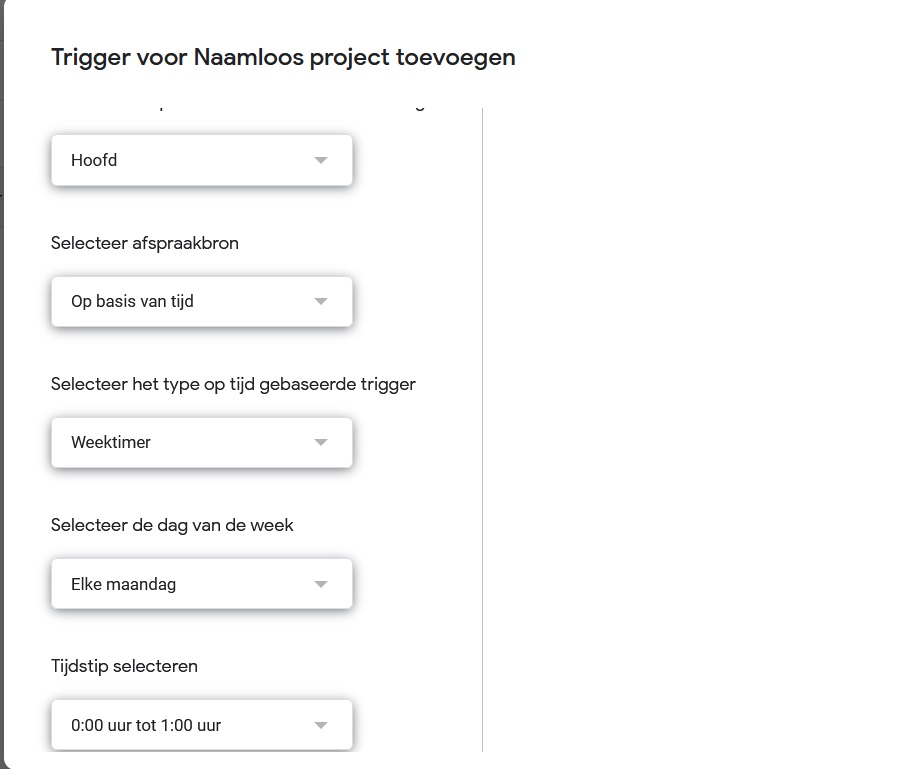
• Create a timer: Within the Apps Script choose the clock icon (left hand) called trigger. Choose "Add Trigger" on the lower right hand corner of the screen.

• At the third drop-down option you can choose "Timer based" and then choose time frame (minutes, day, week... month). Lastly choose the interval.

While creating such script you need to once go through some Google security checkings allowing the script to be executed.

Step 5: Make the graph & upload it to hdashboards

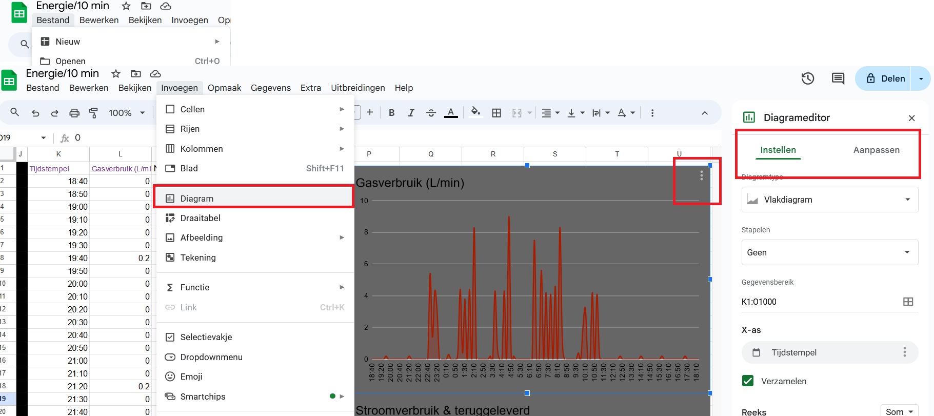
• You can make an graph by using the 'insert' option at the top and choosing graph. After that, you can edit the graph by pressing the 3 dots on the right top of the graph. Everything inside the graph can be adjusted there: the type of graph, the X and Y numbers, the colors, range etc.

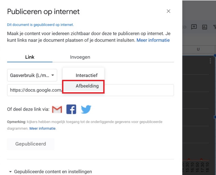
• Once done, you could press the 3 dots on the right top of the graph again and press publish.
• Select Link
• Select the graph you d like to see.
• Select Image
• You ll get an link which you can add into hdashboards by adding an image url.